Data Analytics Final Exam Review
Data pre-processing
Discretization
Binarization
Convert continuous or numerical data into binary values (0, 1) based on some thresholds.
We have listen counts of user and want to determine taste of user. Listen counts is not a robust measure of user taste (Users have different listening habits)
With binarization can transform listen counts into binary values. For example, if listen count >= 10 then map to 1 else map to 0
Binning (Quantization)
Group continuous data into bins (Map continuous data to discrete or categorical one).
- Need to decide bins size (width of each bin)
Here are some interesting methods of binning
Fixed-width binning
Each bin has specific numeric range, it can be any scale (custom designed, automatically segment, linear, exponential)
- Simple
- It may be good on uniformly distributed (fairly even spread)
- Custom Designed : Binning age of people with Stage of life
0 - 12 years old 12 - 17 years old 18 - 24 years old ...
- Exponential-width binning (Relate to Log Transform) : When data has a wide range of values
0 - 9 10 - 99 100 - 999 ...
Fixed-frequency binning
Each interval contains approximately the same number of data points
- When data is not uniformly distributed, we can ensure that each bin contains approximately the same number of data points
Data = [0, 4, 12, 16, 16, 18, 24, 26, 28] Range = (-, 14] [14, 21] [21, +)
Bin 1 : [0, 4, 12] Bin 2 : [16, 16, 18] Bin 3 : [24, 26, 28]
Quantile Binning
Binning base on quantiles (values that divide the data into equal portions)
4-Quantile = Quartiles (Divide data into quarters) 10-Quantile = Deciles (Divide data into tenths)
Steps In K - Quantile = [Q1,Q2,Q3,Q4,...,Qk−1Q_1, Q_2, Q_3, Q_4, ..., Q_k-1] To find position of value of boundary between quantile, find QiQ_i Qi=iK(n+1)th termQ_i = \frac{i}{K}(n+1)^{th} \ term
- K = Number of quantile
- n = Number of data in dataset
- i = Number of Quantile
A lot of empty bins when do fixed width-binning so quantile binning come to help
Data = [1, 1, 1, 2, 2, 3, 4, 4, 10, 10, 10, 500, 1000] Let divide data into Quartiles (4-Quantile) so n = 13 and K = 4
Q1=14(13+1)th=3.5th→1+22=3.5Q_1 = \frac{1}{4}(13+1)^{th} = 3.5^{th} \rightarrow \frac{1 + 2}{2} = 3.5 Q2=24(13+1)th=4th→4Q_2 = \frac{2}{4}(13+1)^{th} = 4^{th} \rightarrow 4 Q3=34(13+1)th=10.5th→10+102=10Q_3 = \frac{3}{4}(13+1)^{th} = 10.5^{th} \rightarrow \frac{10 + 10}{2} = 10Quantile-1 has [1, 1, 1, 2, 2, 3] Quantile-2 has [4, 4] Quantile-3 has [10, 10, 10] Quantile-4 has [500, 1000]
Imbalanced Techniques - Sampling and SMOTE
Imbalanced occur when one class in dataset has more samples than another class. It can be caused by
- Bias while sampling
- Error from measurement
- Natural of that data
Majority Class = Many samples class Minority Class = few samples class
It harder for a model to learn characteristic of Minority Class + some models are assume an equal distribution of class so imbalance can cause problem.
We focus on target variable class
Sampling
Random Under-sampling
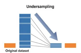
Randomly eliminate samples from majority class until classes distribution balance
When training data is not that small, we can afford under-sampling
Advantages
- Reduce model training time: fewer data points
Disadvantages
- Reduced dataset not represent population or true distribution
- May loss useful data
Random Over-sampling
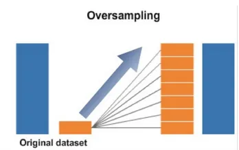
Randomly copy samples in minority class to get more balance distribution
When training data is less, over-sampling would be better than under-sampling
Advantages
- No information loss
Disadvantages
- Overfitting
Synthetic over-sampling: SMOTE
Take subsets of minority class then generate synthetic data points from those subsets and add those new data points to dataset.
It solve overfitting problem of over-sampling
Advantages
- Help with overfitting problem
- No data loss
Disadvantages
- No consideration of majority class
- Addition noise to dataset
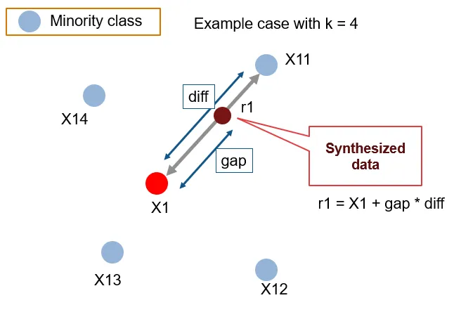
- Finding Nearest Neighbors
- Creating Synthetic Data Points: Do Interpolation
- For each feature dimension, SMOTE calculates a difference value between the selected data point and one of its neighbors.
- It then multiplies this difference by a random value between 0 and 1.
- Finally, it adds this scaled difference to the feature value of the selected data point to create a new synthetic data point.
- Repeat
Dimensional Reduction - PCA
PCA reduces a large number of variables into a set of Principle Component axes.
Why we need to do dimension reduction
Most of the time, we have dataset which has high dimension (many columns or features), we can't visualize those datasets so dimension reduction lend a hand to help with this problem.
Dimension Reduction algorithm will try to preserve all information in higher dimension data and reduce those data into 2-3D where we can visualize and understand(in other word, extract feature out of those high-dimensional data) them.
It can apply prior to applying some models which get affected a lot by Curse of Dimensionality
How to perform PCA
Ref: https://www.youtube.com/watch?v=MLaJbA82nzk
| Feature | ||||
|---|---|---|---|---|
| x | 4 | 8 | 13 | 7 |
| y | 11 | 4 | 5 | 14 |
| Number of features = n = 2 | ||||
| Number of samples = N = 4 |
Features Mean Calculation
xˉ=4+8+13+74=8\bar{x} = \dfrac{4+8+13+7}{4} = 8
yˉ=11+4+5+144=8.5\bar{y} = \dfrac{11+4+5+14}{4} = 8.5
Covariance Matrix Let Ordered Pairs are (x, x) (x, y) (y, x) (y, y)
- Find covariance of all ordered pairs
cov(x,x)==14−1[(4−8)2+(8−8)2+(13−8)2+(7−8)2]=14cov(x, x) = = \dfrac{1}{4-1}[(4-8)^2+(8-8)^2+(13-8)^2+(7-8)^2] =14 cov(x,y)=14−1[(4−8)(11−8.5)+(8−8)(4−8.5)+(13−8)(5−8.5)+(7−8)(14−8.5)]=−11cov(x, y) = \dfrac{1}{4-1}[(4-8)(11-8.5)+(8-8)(4-8.5)+(13-8)(5-8.5)+(7-8)(14-8.5)] =-11 cov(y,y)=cov(x,y)=−11cov(y, y) = cov(x, y) = -11 cov(y,x)=14−1[(11−8.5)2+(4−8.5)2+(5−8.5)2+(14−8.5)2]=33cov(y, x) = \dfrac{1}{4-1}[(11-8.5)^2+(4-8.5)^2+(5-8.5)^2+(14-8.5)^2] = 33
Calculate Eigen value and Eigen Vector then Normalized eigen vector
- Eigen value
where
S=Covariane Matrix=[14−11−1123]I=Identity Matrix=[1001]\begin{align*} S = \text{Covariane Matrix} = \begin{bmatrix} 14 & -11 \\ -11 & 23 \end{bmatrix} \\ I = \text{Identity Matrix} = \begin{bmatrix} 1 & 0 \\ 0 & 1 \end{bmatrix} \end{align*} det(S−λI)=0(14−λ)(23−λ)−(−11×−11)=0λ2−37λ+201=0λ=30.3849, 6.6151→λ1>λ2First Principle Component=λ1=30.3849 and λ2=6.6151\begin{align} \det(S-\lambda I) = 0 \\ (14-\lambda)(23-\lambda)-(-11\times-11) = 0\\ \lambda^2-37\lambda+201=0 \\\\ \lambda = 30.3849,\ 6.6151 \rightarrow \lambda_1>\lambda_2 \\ \text{First Principle Component} = \lambda_1 = 30.3849\ and\ \lambda_2=6.6151 \end{align}- Eigen Vector U1U_1 of λ1\lambda_1
- Normalize the eigen vector U1U_1 get unit eigen vector e1e_1
Derive new dataset
P11=e1T[4−811−8.5]=−4.3052P_11 = e_1^T\begin{bmatrix} 4-8 \\ 11-8.5 \end{bmatrix}=-4.3052 P12=e1T[8−84−8.5]=−4.3052P_12 = e_1^T\begin{bmatrix} 8-8 \\ 4-8.5 \end{bmatrix}=-4.3052| P11 | P12 | P13 | P14 | |
|---|---|---|---|---|
| PC1 | -4.3052 | 3.7561 | 5.6928 | -5.1238 |
Before apply PCA, Standardizing is important step!
- PCA seeks to maximize the variance of each component and Standardizing is a variance maximizing exercise
Model Evaluation
Cross-Validation
Technique to evaluate predictive models by partitioning the original sample into a training set to train the model and a test set to evaluate it.
There are many interesting methods those use cross-validation technique.
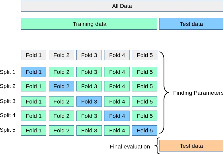
We can also use the cross validation set to tune model hyperparameters and test with test set later.
Holdout method
Separate dataset into two sets training set and testing set
- Use training set to train only and then predict testing set and validate the model on it
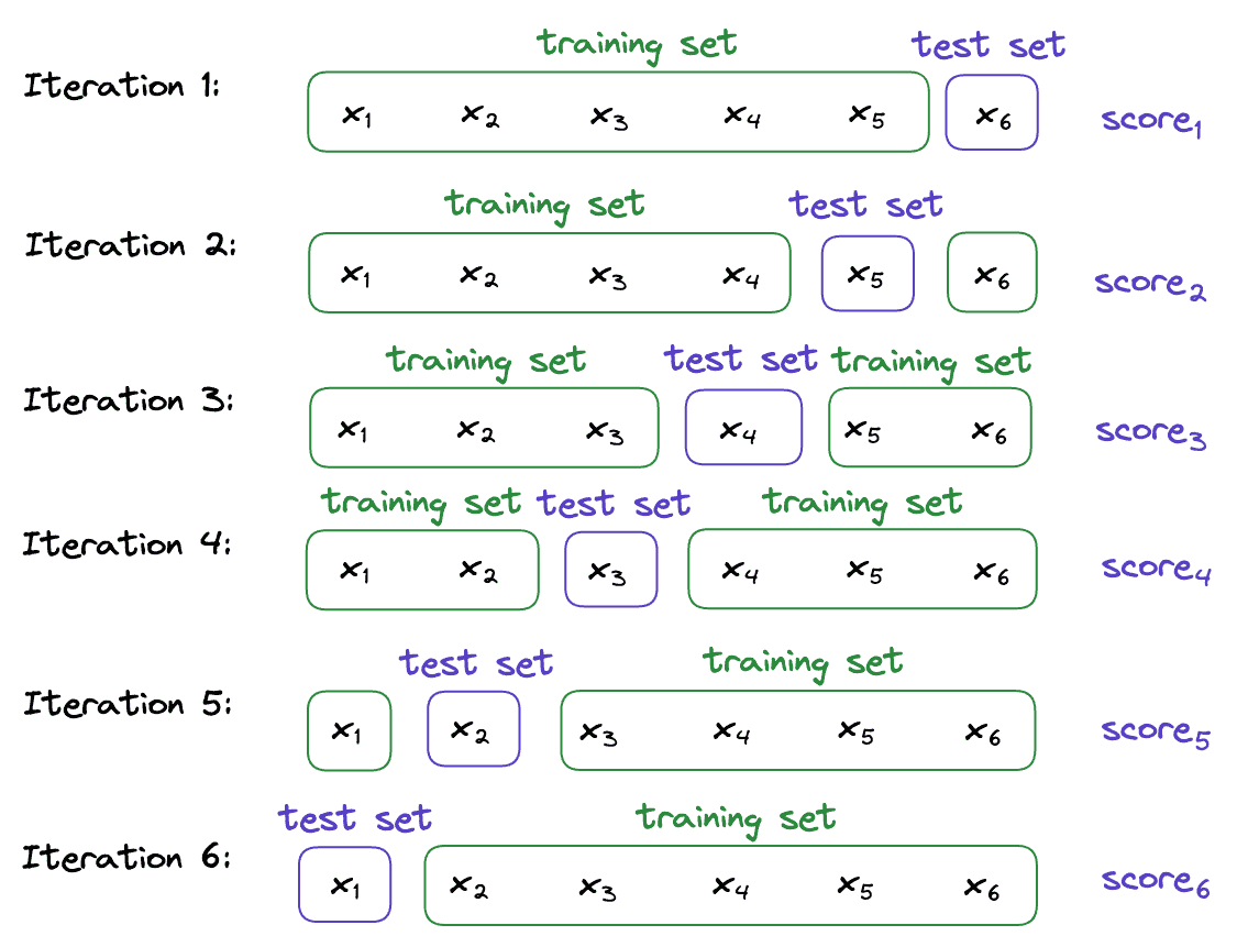
K-fold cross validation
Randomly divide dataset into K equal-size parts, X1 X2 X3 ... XkX_1\ X_2\ X_3\ ...\ X_k, use K-1 part as training set and the left one is Validation set
Advantage
- Good to use when don't have a large enough dataset (When a single, random sample of the data is not representative sample of the underlying distribution)
**Disadvantage
- K have effect, larger K →\rightarrow larger training sets that overlap more, leading to a stronger dependence between the results in the K folds
- Expensive computational time
Leave-one-out cross validation
Extreme case of K-fold cross validation, only one sample is used as a Validation set while the rest are used to train our model
Partitioning Clustering
Data clustering concept
- Grouping similar data points together based on certain criteria
- Unsupervised Learning
- Use Distance/Similarity Metric
The goal of clustering is to discover natural groupings or clusters in the data without any prior knowledge of the groupings.
Pre-processing for clustering
- Normalize the data
- Remove noises or outliers
- Approach few numbers of dimensions (dimensional reduction)
K-means
How to perform K-means
Let A1=(3,8), A2=(9,4), A3=(4,9), A4=(2,2), A5=(10,5), A6=(2,4), A7=(6,8), A8=(4,3), A9=(4,7)\text{A1=(3,8), A2=(9,4), A3=(4,9), A4=(2,2), A5=(10,5), A6=(2,4), A7=(6,8), A8=(4,3), A9=(4,7)}

In this problem we will use K=3K=3
Goal: Find member and centroid of each cluster
Step
- Choose K-centroid randomly (It can be any points)
- Find the nearest centroid cjc_{j} for each point and assign each point to those centroid
In this problem we use Euclidean Distance
Distance(A,B)=(AX−BX)2+(AY−BY)2\text{Distance}(A, B) = \sqrt{ (A_{X} - B_{X})^2 + (A_{Y} - B_{Y})^2 }Let assume that we have assigned each point to its nearest centroid using Euclidean distance as a matric distance and get this result.
- j1 has [A1, A3, A7, A9]
- j2 has [A4, A6, A8]
- j3 has [A2, A5]
- Find new centroid cjc_{j} and see if cluster member change or not
- If cluster member remain the same : Finish!
- If cluster member change : Find new centroid again!
from j = 1 to K
cj(X)=1n∑i=1nxicj(Y)=1n∑i=1nyicj=(cj(X), cj(Y))\begin{align} c_{j}(X) = \dfrac{1}{n}\sum_{i=1}^{n}x_{i} \\ c_{j}(Y) = \dfrac{1}{n}\sum_{i=1}^{n}y_{i} \\\\ c_{j} = (c_{j}(X),\ c_{j}(Y)) \end{align}where
n=Number of points in cluster with centroid cjxi=X coordinate of Point in cluster with centroid cjyi=Y coordinate of Point in cluster with centroid cj\begin{align} n = \text{Number of points in cluster with centroid } c_{j} \\ x_{i} = \text{X coordinate of Point in cluster with centroid } c_{j} \\ y_{i} = \text{Y coordinate of Point in cluster with centroid } c_{j} \end{align}Example
| j | cj(X)c_{j}(X) | cj(Y)c_{j}(Y) | centroid cjc_{j} |
|---|---|---|---|
| 1 | 3+4+5+64=4.25\dfrac{3+4+5+6}{4}=4.25 | 8+9+8+74=8\dfrac{8+9+8+7}{4}=8 | (4.25, 8)(4.25,\ 8) |
| 2 | 2+2+43=2.667\dfrac{2+2+4}{3}=2.667 | 4+3+23=3\dfrac{4+3+2}{3}=3 | (2.667, 3)(2.667,\ 3) |
| 3 | 10+92=9.5\dfrac{10+9}{2}=9.5 | 4+52=4.5\dfrac{4+5}{2}=4.5 | (9.5, 4.5)(9.5,\ 4.5) |
- j1 has [A1, A3, A7, A9]
- j2 has [A4, A6, A8]
- j3 has [A2, A5]
Member of cluster is not changed so FINISH!
Result

Clustering Evaluation
Elbow Method
Help choose the right number of clusters for your clustering algorithm by plot graph between the number of clusters and the sum of squared distances
Within Cluster Sum of Squares - WCSS
WCSS=Sum of distance between each point its centroid in each clusterWCSS = \text{Sum of distance between each point its centroid in each cluster} WCSS=∑P in Cluster 1distance(Pi,C1)2+…WCSS = \sum_{\text{P in Cluster 1}}distance(P_{i}, C_{1})^2 + \dotsthen plot on graph where y is WCSS and x is Number of clusters
Association Rule
Apriori Algorithm
Ref: https://www.youtube.com/watch?v=rgN5eSEYbnY
Goal : get frequent itemset which is a set of data that tend to happen together.
Step
| Customer ID | Transaction ID | Item Bought |
|---|---|---|
| 1 | 0001 | {a, d, e, f} |
| 1 | 0024 | {a, b, c, e} |
| 2 | 0012 | {a, b, d, e} |
| 2 | 0031 | {a, c, d, e} |
| 3 | 0015 | {b, c, e} |
| 3 | 0022 | {b, d, e} |
| 4 | 0029 | {c, d} |
| 4 | 0040 | {a, b, c} |
| 5 | 0033 | {a, d, e} |
| 5 | 0038 | {a, b, e} |
| Let minimum support 40% |
- Filter item with minimum support
Filter out the item which Support < Minimum support
| Transaction ID | a | b | c | d | e | f |
|---|---|---|---|---|---|---|
| 0001 | 1 | 1 | 1 | 1 | ||
| 0024 | 1 | 1 | 1 | 1 | ||
| 0012 | 1 | 1 | 1 | 1 | ||
| 0031 | 1 | 1 | 1 | 1 | ||
| 0015 | 1 | 1 | 1 | |||
| 0022 | 1 | 1 | 1 | |||
| 0029 | 1 | 1 | ||||
| 0040 | 1 | 1 | 1 | |||
| 0033 | 1 | 1 | 1 | |||
| 0038 | 1 | 1 | 1 | |||
| Count | 7 | 6 | 5 | 6 | 8 | 1 |
| 10 | 10 | 10 | 10 | 10 | 10 | |
| Support | 70% | 60% | 50% | 60% | 80% | 10% |
| Pass? | ✅ | ✅ | ✅ | ✅ | ✅ | ❌ |
- Create itemset
To create itemset
2-Itemset
| Product | Support | Pass? | ||
|---|---|---|---|---|
| {a, b} | 4 | 10 | 40% | ✅ |
| {a, c} | 3 | 10 | 30% | ❌ |
| {a, d} | 4 | 10 | 40% | ✅ |
| {a, e} | 6 | 10 | 60% | ✅ |
| {b, c} | 3 | 10 | 30% | ❌ |
| {b, d} | 2 | 10 | 20% | ❌ |
| {b, e} | 5 | 10 | 50% | ✅ |
| {c, d} | 2 | 10 | 20% | ❌ |
| {c, e} | 3 | 10 | 30% | ❌ |
| {d, e} | 5 | 10 | 50% | ✅ |
3-Itemset
| Product | Support | Pass? | ||
|---|---|---|---|---|
| {a, b ,c} | 4 | 10 | 40% | ✅ |
| {a, c, d} | 1 | 10 | 10% | ❌ |
| {a, d, e} | 4 | 10 | 40% | ✅ |
| {b, c, e} | 2 | 10 | 20% | ❌ |
| ... | ... | ... | ... | ... |
4-Itemset
| Product | Support | Pass? | ||
|---|---|---|---|---|
| {a, b ,c, e} | 1 | 10 | 10% | ❌ |
| {a, b, d, e} | 1 | 10 | 10% | ❌ |
| {a, c, d, e} | 1 | 10 | 10% | ❌ |
| ... | ... | ... | ... | ... |
- Get Association Rule and Calculate Confidence and Lift
Association define as
A→BA \rightarrow BIf A exist in transaction then B tend to exist too. For example, If Customer 1 buy A then he tend to buy B too.
We usually call
A:AntecedentB:Consequent\begin{align} A : Antecedent \\ B : Consequent \end{align}| Antecedent | Consequent | Association Rule |
|---|---|---|
| {b} | {a, d, e} | {b}→{a,d,e}\{b\} \rightarrow \{a, d, e\} |
| {a, d, e} | {b} | {a,d,e}→{b}\{a, d, e\} \rightarrow \{b\} |
| ... | ... | ... |
Confidence
confidence(A→B)=Support(A, B)Support(A)Support(A→B)=Frequecy(A,B)N \boxed{ \ \begin{align} \\ \text{confidence}(A \rightarrow B) = \dfrac{\text{Support}(A,\ B)}{\text{Support}(A)} \\\\ \text{Support}(A \rightarrow B) = \dfrac{\text{Frequecy}(A, B)}{N} \\ \\ \end{align}\ }Measures how often a rule is true
- if A occurs, B is likely to occur
Minimum Confidence set a minimum line for confidence
Let say, minimum confidence = 0.2
| Association Rule | Support(A, B) | Support(A) | Confifence(A →\rightarrow B) | Pass Minimum Confidence |
|---|---|---|---|---|
| {b}→{a,d,e}\{b\} \rightarrow \{a, d, e\} | Support({b},{a,d,e})=110Support(\{b\} , \{a, d, e\}) = \dfrac{1}{10} | Support({b})=610Support(\{b\}) = \dfrac{6}{10} | 110×106=16\dfrac{1}{10}\times \dfrac{10}{6} = \dfrac{1}{6} | ❌ |
| {a,d,e}→{b}\{a, d, e\} \rightarrow \{b\} | Support({a,d,e},{b})=110Support(\{a, d, e\} , \{b\}) = \dfrac{1}{10} | Support({a,d,e})=410Support(\{a, d, e\})=\dfrac{4}{10} | 110×104=14\dfrac{1}{10}\times \dfrac{10}{4} = \dfrac{1}{4} | ✅ |
| ... | ... | ... | ... | ... |
Lift
Lift(A,B)=Support(A,B)Support(A)×Support(B)\boxed{\text{Lift}(A, B) = \dfrac{\text{Support}(A, B)}{Support(A)\times Support(B)}}Measure of the strength of the association between two items
- Lift greater than 1 indicates that the presence of item A has a positive effect on the presence of item B
Decision Trees and Random Forest
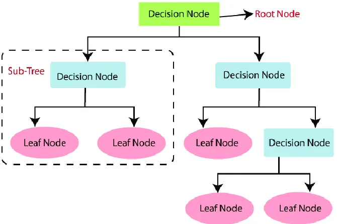
Terminology
Node Impurity
Node is like a dataset or subset of data in decision tree. Pure Node is a subset where all samples are in the same class
| A | B | Class |
|---|---|---|
| 1 | 22 | + |
| 22 | 3213 | + |
| 12 | 32 | + |
Impure Node is a subset where samples has same portion of classes (#Class + = #Class -)
Entropy
Entropy of a random variable is the average level of "information", "surprise", or "uncertainty" inherent to the variable's possible outcomes
When we measure entropy of something, it like we measure how much information we need to describe that thing or measure randomness in the system
In decision tree algorithm, entropy measure impurity in the Node
- Pure Node: entropy = 0 (no impurity + need only few information to describe that node) →\rightarrow low randomness
Example
Find entropy of this Node S where class label are + and -.
| Height | Race | Sex | Class |
|---|---|---|---|
| 160 | Asian | F | + |
| 170 | Hispanic | F | + |
| 180 | White | M | - |
| 170 | White | M | + |
| 180 | Asian | M | - |
| Probability that person will be + is 3/5 = 0.6 | |||
| Probability that person will be - is 2/5 = 0.4 |
NOTE: when Pi=0P_{i} = 0, entropy = 0 ()
Information Gain
In decision tree, information gain measure how much entropy will be reduced after each split
- Compute the difference between entropy before split and average of entropy after the split
- Less reduction of entropy →\rightarrow More Information Gain
Information gain help us select best feature to use to split the data at each internal node of the decision tree
- Feature with the highest information gain is chosen as the split feature
Example
Let use the previous example where Entropy(S)=0.970951Entropy(S) = 0.970951
| Height | Race | Sex | Class |
|---|---|---|---|
| 160 | Asian | F | + |
| 170 | Hispanic | F | + |
| 180 | White | M | - |
| 170 | White | M | + |
| 180 | Asian | M | - |
| Find Information Gain of Sex or GAIN(S, Sex) | |||
| Value(Sex)=Value(Sex)= {F, M} | |||
| SF=S_{F}= 2 {2+, 0-} | |||
| SM=S_{M}= 3 {1+, 2-} | |||
| SS = 5 {3+, 2-} | |||
| Entropy(S)=Entropy(S)= 0.970951 | |||
| Entropy(SF)=0Entropy(S_{F})=0 | |||
| Entropy(SM)=−(13log213)−(23log223)=0.9182Entropy(S_{M})=-(\dfrac{1}{3}\log_{2}{\dfrac{1}{3}})-(\dfrac{2}{3}\log_{2}{\dfrac{2}{3}})= 0.9182 |
GINI Index
GINI index also measure the impurity, it is like information gain but compute differently (GINI faster to compute)
GINI(E)=1−∑j=1Cpj2\boxed{ GINI(E) =1 - \sum_{j=1}^{C}p_j^2 }| Height | Race | Sex | Class |
|---|---|---|---|
| 160 | Asian | F | + |
| 170 | Hispanic | F | + |
| 180 | White | M | - |
| 170 | White | M | + |
| 180 | Asian | M | - |
Example
Find GINI index of Sex
F=F= 2 {2+, 0-} M=M= 3 {1+, 2-} SS = 5 {3+, 2-}
GINI(F)=0GINI(F)=0 GINI(M)=1−((13)2+(23)2)=1.3333..GINI(M)=1-((\dfrac{1}{3})^2 +(\dfrac{2}{3})^2) =1.3333..
For continuous values, we need to apply discretization first.
Decision Trees
Decision Trees construction
Too lazy laew, doo this one https://www.youtube.com/watch?v=_L39rN6gz7Y
Steps
Parameters
- Max Depth: Maximum depth of the tree
- Higher depth: Lead to overfit
- Min Sample Split: Minimum sample require to split an internal node
- Prevent splitting with too few sample
- Min Sample Leaf: Minimum sample require to be leaf node
- Prevent overfitting
- Max Features: Maximum number of features to consider when splitting a node
- Criterion: GINI, Entropy
Random Forest
Pick a random subset S, of training samples
- For each subset => grow a full tree
- Given, a new data point X
- Classify X using each of the trees
- For example, use majority vote: class predicted most often
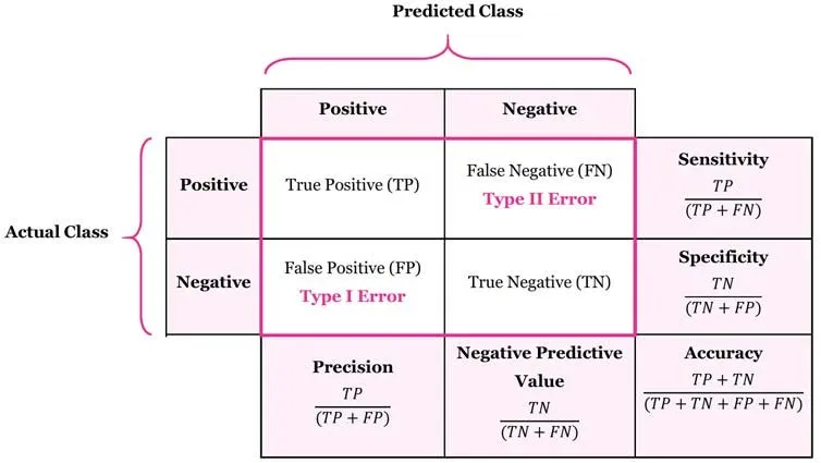
Evaluation
Decision Tree is mainly use as classifier so we can use Evaluate with Precision/Recall, F-Score and Confusion Matrix
Recommenders Systems
Information filtering system that implicitly or explicitly capture a user's preference and generate a ranked list of items that might be of interest to the user.