UMAP - How does it work?

What is UMAP §

Uniform Manifold Approximation and Projection or UMAP is s a dimension reduction technique used for visualizing data based on manifold learning method.

It constructs a high-dimensional graph representation of the data and then optimizes a low-dimensional graph to be structurally similar. This method is similar to t-SNE but offers a more general framework for manifold learning and dimension reduction.

Why we need to do dimension reduction? §

Most of the time, we have dataset which has high dimension (many columns or features), we can’t visualize those datasets so dimension reduction lend a hand to help with this problem.

Dimension Reduction algorithm will try to preserve all information in higher dimension data and reduce those data into 2-3D where we can visualize and understand(in other word, extract feature out of those high-dimensional data) them.

It can apply prior to applying K-nearest-neighbors algorithm which get affected a lot by Curse of Dimensionality

How does UMAP work? §

To understand math of UMAP, we need to understand these concepts first.

Manifold Learning §

Usually, Manifold Learning consist of these same steps^[https://youtu.be/YevCnRd61f8?t=813]

1. Choose distance metric
2. Build k-nearest-neighbor graph
3. Weight that neighbor graph
4. Symmetrize that neighbor graph
5. Embed that graph into a metric space

Topological Space, Simplex, Simplicial Complexes and other Mathematic terms §

Topology is a way we study space that involve things like connectedness, dimension instead of area, length, etc. (geometry)

when we interested in objects A, B, C and relationship between them (Morphism) $A\to B$ for example, in algebra objects are groups and morphisms between them are group homomorphism. in linear algebra objects can be vector spaces and morphisms are linear map.

In topology, objects are topological spaces and the morphisms between them are continuous function.

Topological Space is the most general type of space in mathematic that allow definition of 1. limit 2. continuity 3. connectedness

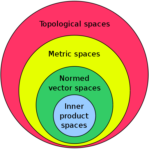
Maybe we’ve already know Metric spaces and Normed vector spaces, those spaces are subset of Topological Spaces

In other word, in metric space, we can calculate distance (metrizable, we can define a matric in that topological space so it is metric space)

Topological spaces only have notion of closeness without metric, there are some topological spaces those aren’t metric space but all metric spaces are topological spaces.

Manifold is a topological space that look like a Euclidean space when we zoom in enough for example, earth is sphere which is curved but if we look close enough we can see sphere as a plane (earth map).

in other word, topological manifolds must be locally homeomorphic (preserve all the topological properties of a given space) to Euclidean space

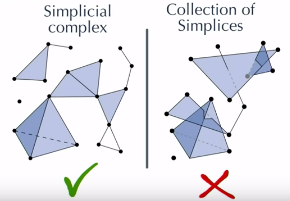
Simplex is a very simple way to build k-dimensional object.

Simplicial Complexes is any 2 simplices are either disjoint or meet in a common face

In other word, to construct simplicial complexes, we need to glue together simplices of various dimensions along their faces.

Q: What are faces of simplex? A: Let S is a simplex number 1 and P is a simplex number 2 then face is $P$ where $P\subset S$ whose vertices of P are also vertices of S

Cover, Open Cover and Čech complex §

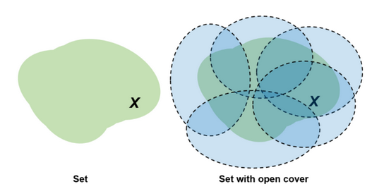
Cover Let $A$ is a set and $B$ is Union of a bunch of sets $A=[0,3]$ $B=Union\{[0,2],(1,4),[5,7)\}$

Then $B$ is cover of A when $A\subset B$

Open Cover It is like a cover but each sets in B need to be open set

$A=[1,2]$ $B=Union\{(0,2),(1,4),(5,7)\}$

Then $B$ is open cover of A when $A\subset B$, where all sets from B are open set

Čech complex to covert open cover into simplicial complex we need Čech complex. Process to build it is very simple

• let each set in the cover be a 0-simplex
• create 1-simplex between two sets if they have a non-empty intersection (overlap), create a 2-simplex between three such sets if the triple intersection of all three is non-empty and so on.

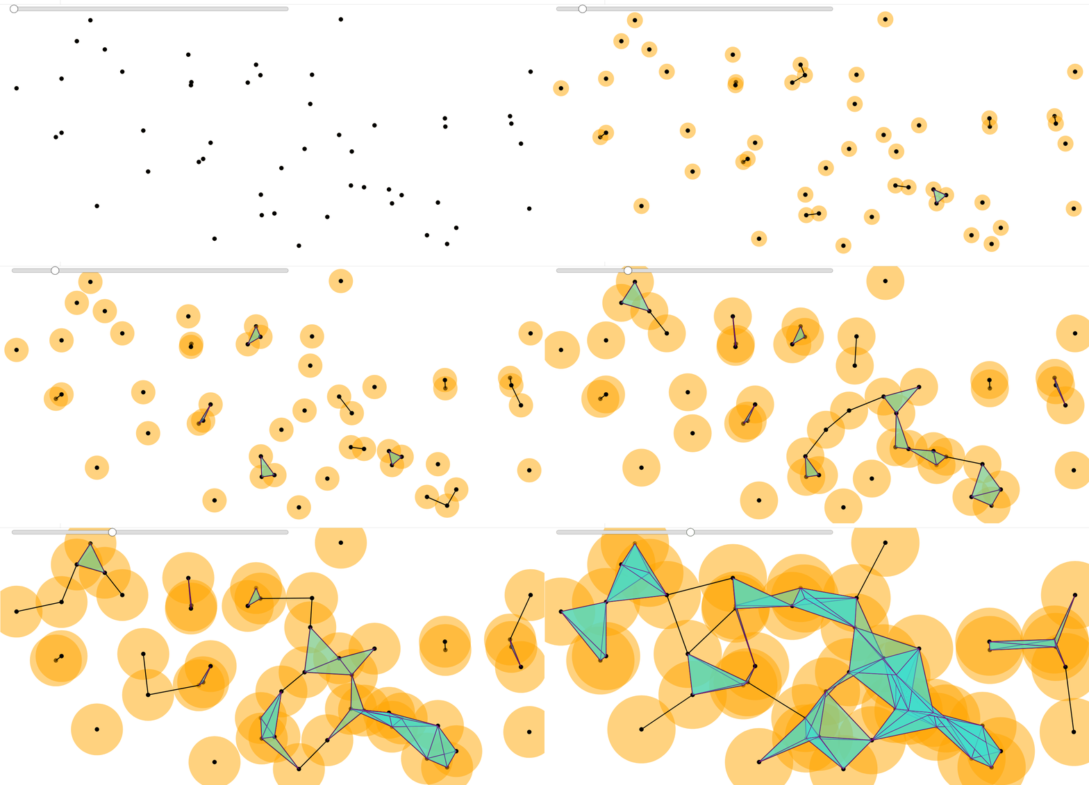
for visualization, visit Čech Complex Playground

Note

There is a theorem that will make sure that process to build Čech Complex will produce something that represents the topological space itself in a meaningful way.

It is Nerve Theorem : If we build simplicial complex out of topological space in that certain way, we can actually recover all the important topology of that space

Use those concept with real finite data samples §

To learn about topology of the data samples, we need to apply process of Čech complex to our data. Before that, we need to generate an open cover so we can turn it into simplicial complex.

so how can we generate open cover?

we can simply create balls of some fixed radius about each data points, anyway, we don’t sure if those balls are open cover or not but it is best approximation we can make. Then, we build simplicial complex out of it.

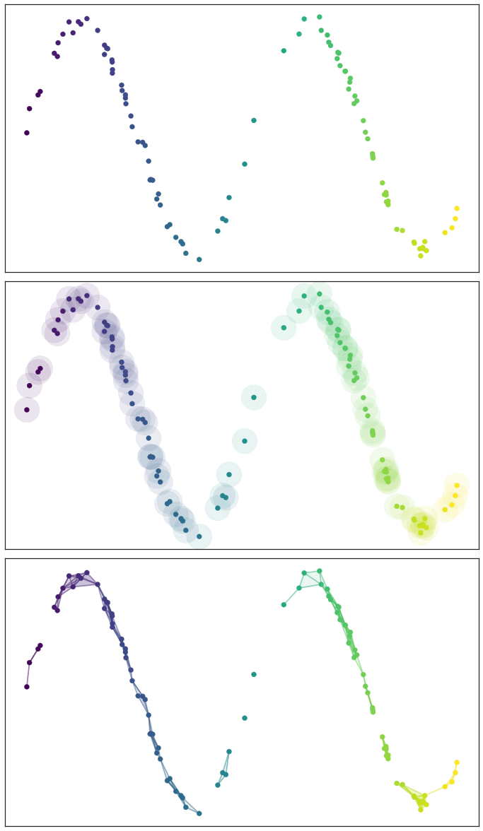
We can find a low dimensional representation of the data that has similar topological representation.

But we can see that there are a lot of gaps between many data points, if data points are uniformly distributed on the manifold, that would be great. So we need to make first assumption.

1. Data is uniformly distributed on the manifold

But! real data’s don’t usually work work like that! will it work? Yes, because we’ve already assume that Data is uniformly distributed on the manifold so we can ask about that manifold that data is distributed on instead.

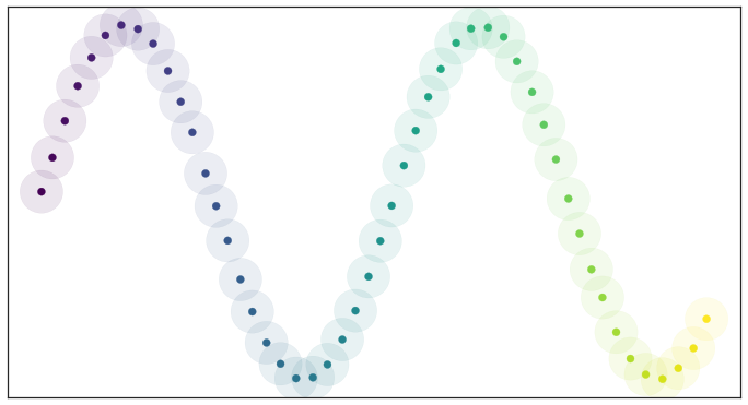
so we need to define a Riemannian metric on the manifold to make this assumption true. Defining a Riemannian metric on a manifold is like equip manifold with measuring tool that works specifically for that space.

Note

So we need to ask about that manifold that data is distributed on instead (because real data doesn’t behave in a good way)

From UMAP paper, author use idea that we create Balls $B$ those center at point $p$ where both volume and geodesic distance from center $p$ to any point $q\in B$ respect to Riemannian metric which this metric locally constant about $p$ on Manifold .

With this idea and assumption number 1, any of those balls should contain the same number of points.

And from the idea of locally metric constant and ball center at some points $p$ contain approximately same amount of points (its k-nearest neighbors of that points $p$) , then, we can find distance from $p$ to those neighbors where those geodesic distance is vary depend on neighbors of $p$ (Each point has its own unique distance function).

[!NOTE 2 | NOTE]

From presentation by author of UMAP at 8:05, he say that we define Riemannian metric on the manifold that make assumption I magically true by vary notion of distance on manifold (There exist a lot of patches glued together that map manifold to Euclidean space on different scales).

From metric we define above, we get our second assumption for UMAP

2. UMAP assume that the Riemannian metric is locally constant, or can be approximated as such.

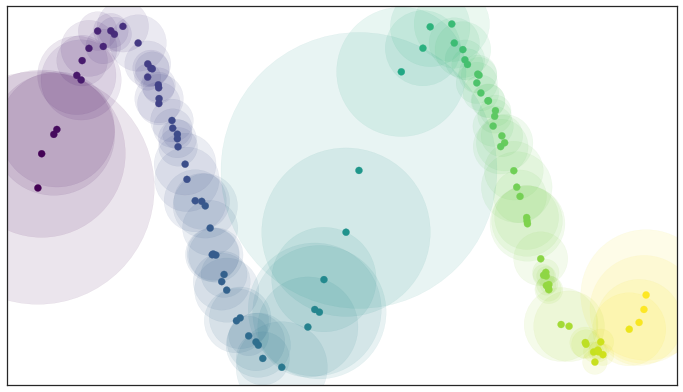
“All of those balls have same size as far a distance on the manifold is concerned, it’s a different in Euclidean Space, but for the manifold we claim that our data lie on, these ball are the same size”^[https://youtu.be/nq6iPZVUxZU?t=566]

Fuzzy topology (No more fixed distance) §

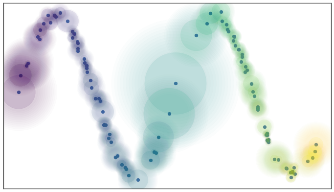
Instead of fixed radius of each balls, we can look it in a fuzzy way, in other meaning, if we’re considering points within a certain radius from a center point, the certainty that a point is within that radius decreases as we move farther away from the center (not 0 or 1 but 0 to 1). There is mathematical way to do this cleanly call UMAP Adjunction

and here is the result.

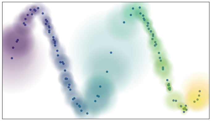
but there are some isolated points when we process data this way, so the third assumption is made to assure that any points on manifold have neighbor (no isolated points).

3. The manifold is locally connected

Local connectivity make the distribution of normalized distance in higher dimension look like one in lower dimension

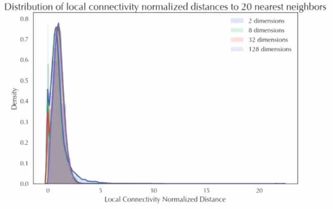From UMAP Uniform Manifold Approximation and Projection for Dimension Reduction | SciPy 2018 |

It effective way to work with curse of dimensionality in high dimensions data where high dimensions distances tend to be larger, but also more similar to one another.

Local metrics is incompatible! §

There is one problem we need to solve! Because each point has its own metric so there are many distance from point to point to use. For example, distance from point $A$ to $B$ is 100 but in perspective of $B$, $B$ to $A$ is 50, which one to choose?

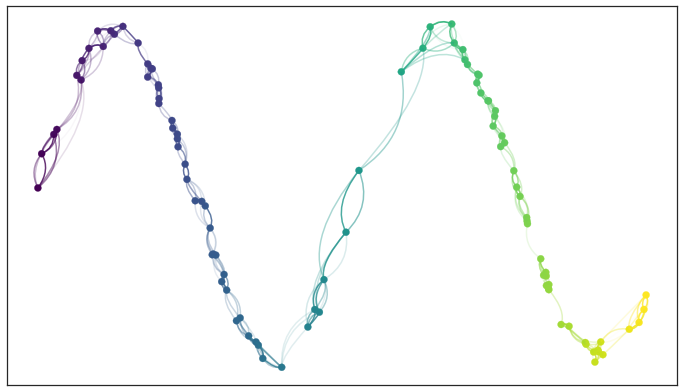
We might create two weight edges for each pair of point, those edges are disagree with each other and we will combine weight with this formula

$f(a,b)=a+b-a\cdot b$

and we end up with this weighted graph

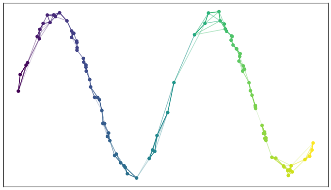(fuzzy topological representation of the data which capture the topology of the manifold underlying the data )

Covert into Low Dimensional Representation §

Goal is to preserve shape of fuzzy topological structure as much as possible

We can apply same process to create that fuzzy topological graph, what does we need to know and do to create that?

• Manifold (in high dimensional, we inferred it but! in low dimensional such as 2D or 3D manifold is $R^2$ and $R^3$)
• Best k-nearest-neighbors (This is hyperparameter) Suppose we’ve already get this new low representation graph, how can we find similarity between two fuzzy topological graph, we will use Cross Entropy

Let E be set of all 1-simpleces ${\sum }_{e\in E}{w}_h(e)\log \left(\frac{w_h(e)}{w_l(e)}\right)+(1-w_h(e))\log \left(\frac{1-w_h(e)}{1-w_l(e)}\right)$ where $w_h(e)$ and $w_l(e)$ is weight of the 1-simplex $e$ in high or and dimension while

First Term ${\sum }_{e\in E}{w}_h(e)\log \left(\frac{w_h(e)}{w_l(e)}\right)$ this term will adjust the clump.

Second Term $(1-w_h(e))\log \left(\frac{1-w_h(e)}{1-w_l(e)}\right)$ this term will adjust the gaps.

Summary §

1. Construct weighted graph by patching together local view of manifold that map to Euclidean space.
2. Use cost function and optimizer to optimize over low dimension fuzzy topological structure aim to get structure that preserve topological shape of data in high dimensional.

UMAP Algorithm §

UMAP algorithm has these simple steps

1. Construct the weighted graph
2. Perform optimization of the graph layout

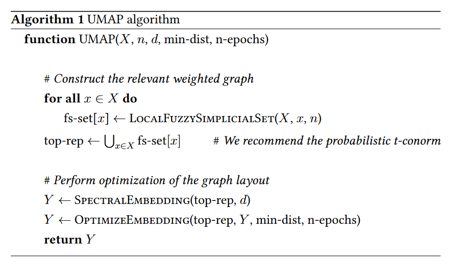
Algorithm aim to preserve overall topology of the source data.

Hyperparameters Tuning §

UMAP has so many parameters we can custom but in this section, we will select only some important parameters.

import umap
 
umap = UMAP(
	n_neighbors=10,
	n_components=1,
	min_dist=0.1,
)

n_neighbors §

• Control over k-nearest-neighbors
• Decrease for more local structure
• Increase for smoother embedding

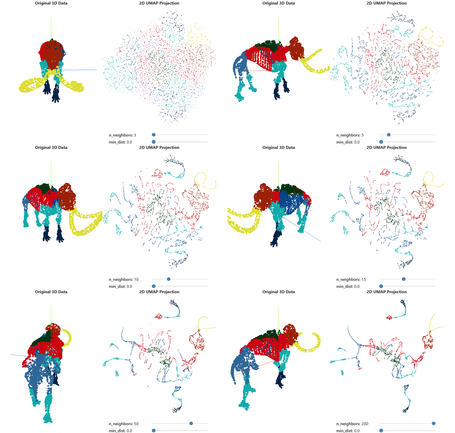^[https://pair-code.github.io/understanding-umap/]

min_dist §

• Smaller values: Emphasize local structure, potentially forming tighter clusters.
• Larger values: Spread points out more uniformly.

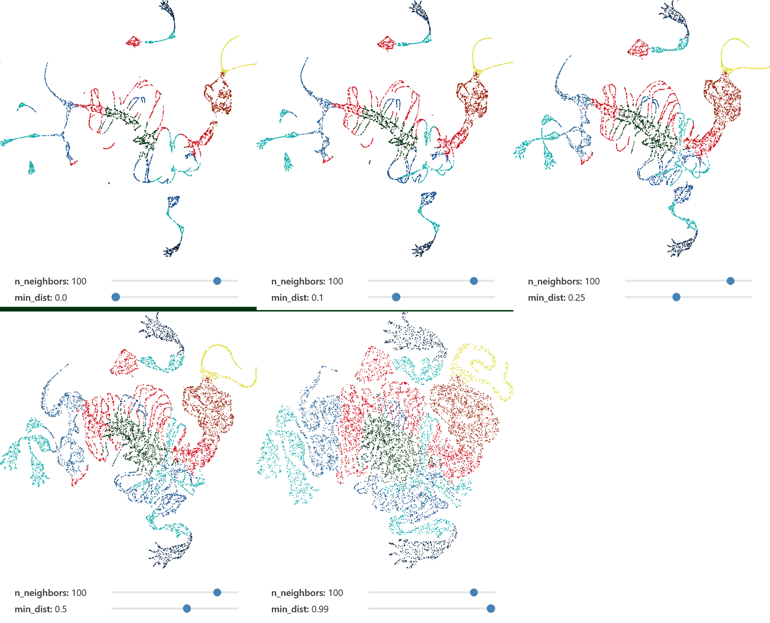
n_components §

Typically set to 2 for visualization. Experiment with 3 for specific applications

References §

1. McInnes, L., Healy, J., & Melville, J. (2018, February 9). UMAP: Uniform Manifold Approximation and Projection for Dimension Reduction. arXiv.org. https://arxiv.org/abs/1802.03426
2. How UMAP Works — umap 0.5 documentation. (n.d.). https://umap-learn.readthedocs.io/en/latest/how_umap_works.html
3. L. (2018, June 13). Notes on Topology. LoganThrasherCollins.com. https://logancollinsblog.com/2017/11/12/notes-on-topology/
4. I. I. M. (2012, October 7). Simplices and simplicial complexes | Algebraic Topology | NJ Wildberger. YouTube. https://www.youtube.com/watch?v=Uq4dTjHfLpI
5. Understanding UMAP. (n.d.). https://pair-code.github.io/understanding-umap/
6. E. (2018, July 13). UMAP Uniform Manifold Approximation and Projection for Dimension Reduction | SciPy 2018 |. YouTube. https://www.youtube.com/watch?v=nq6iPZVUxZU
7. P. (2019, February 1). A Bluffer’s Guide to Dimension Reduction - Leland McInnes. YouTube. https://www.youtube.com/watch?v=9iol3Lk6kyU
8. J. T. T. V. (2022, August 28). What is Topology? YouTube. https://www.youtube.com/watch?v=WdIVpbOKyM8
9. B. T. (2021, November 24). BioTuring Webinar: A Practical Guide to UMAP by its author John Healy. YouTube. https://www.youtube.com/watch?v=YevCnRd61f8