Design a simplified Google Maps. Google Maps has 1B DAU, 99% world coverage, 25M location updates daily. Focus on: location update, navigation (including ETA), and map rendering. Primary devices: mobile phones.

Step 1 - Understand the Problem and Establish Design Scope

Key features #

1. User location update.
2. Navigation service (including ETA).
3. Map rendering.

Support driving, walking, bus modes. Multi-stop directions out of scope. Traffic conditions important for accurate ETA. Road data: TBs of raw data from external sources.

Non-functional requirements #

• Accuracy: no wrong directions.
• Smooth navigation: smooth map rendering on client.
• Data and battery: minimal data/energy usage on mobile.
• General scalability and availability.

Map 101 #

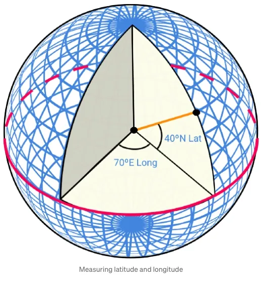
Positioning: Latitude (north/south), Longitude (east/west).

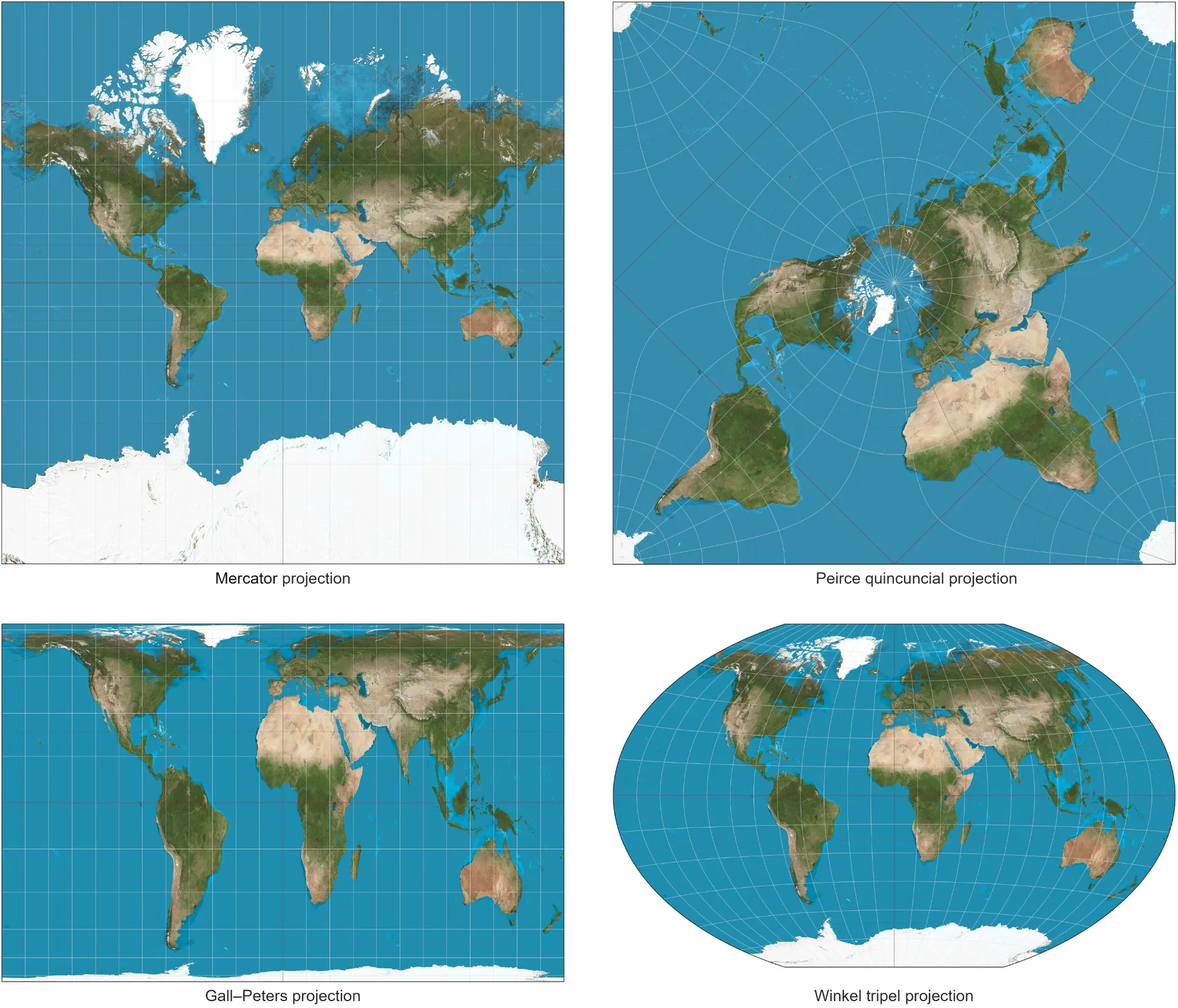
Map projection: 3D globe → 2D plane. Google Maps uses Web Mercator (modified Mercator).

Geocoding: Address → lat/lng (e.g., "1600 Amphitheatre Parkway, Mountain View, CA" → 37.423021, -122.083739). Reverse geocoding: lat/lng → address. Uses interpolation from GIS data.

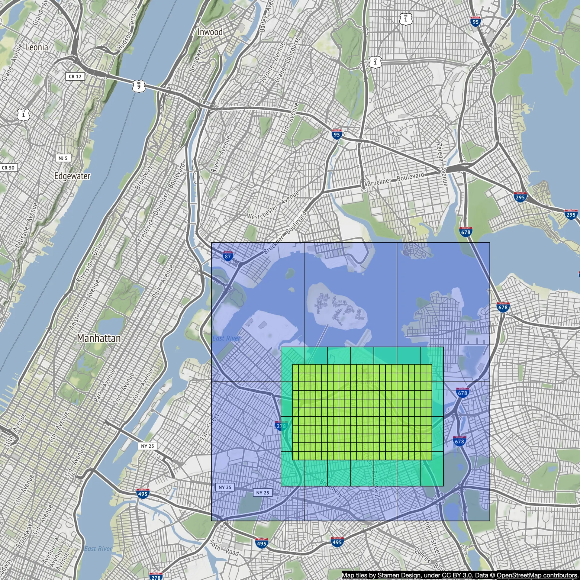
Geohashing: Encodes geographic area into short string. Recursively divides grids into sub-grids. Used for map tiling in this design.

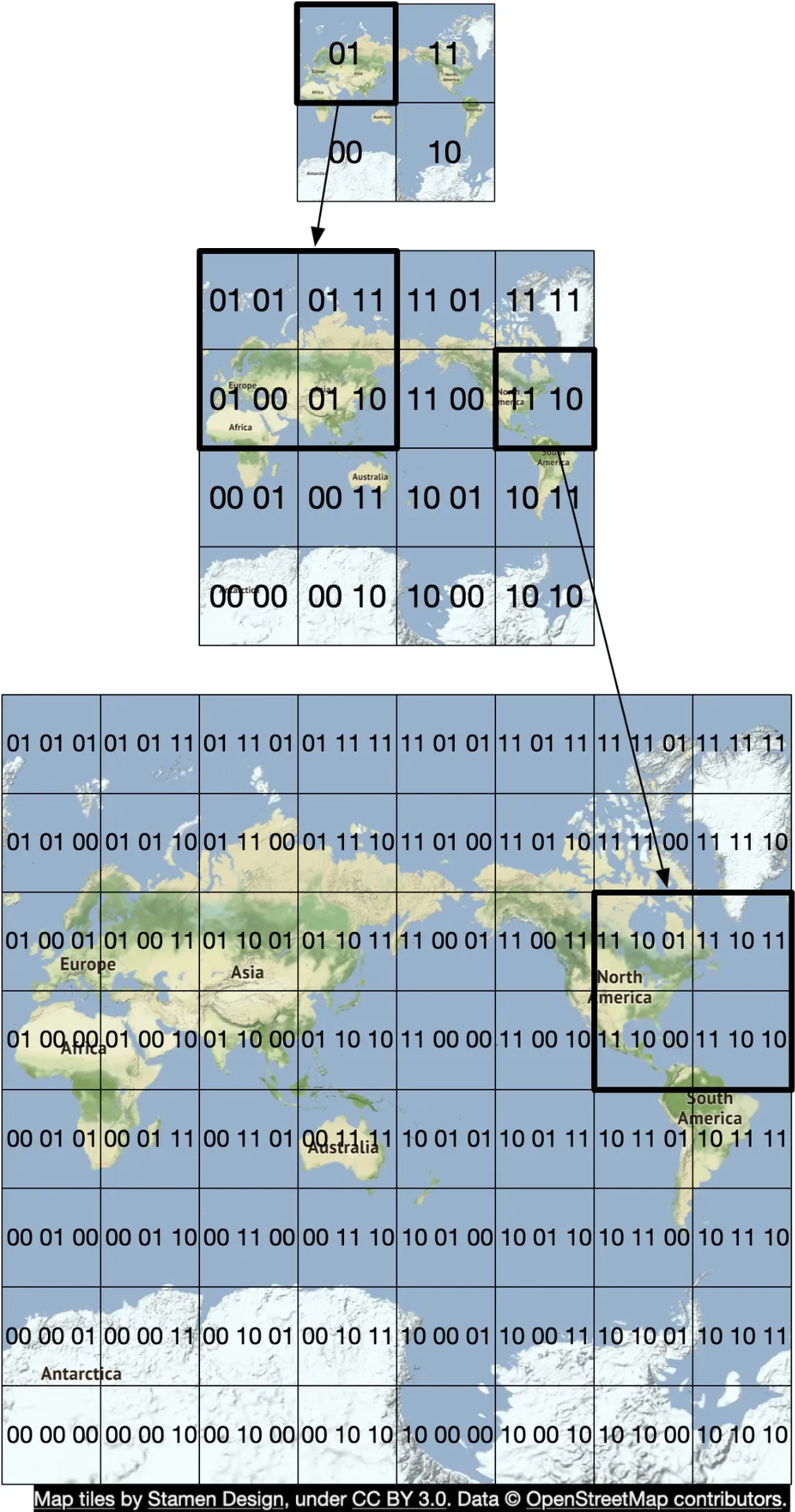
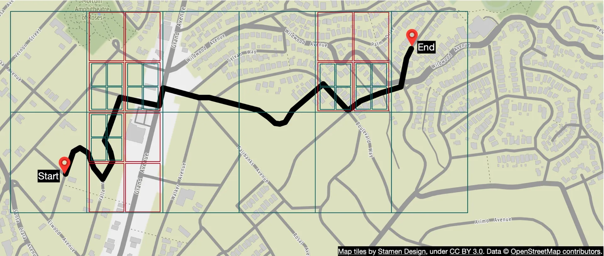
Map rendering: World broken into tiles (256×256 px PNGs at different zoom levels). Client downloads only relevant tiles for viewport + zoom level, stitches them together.

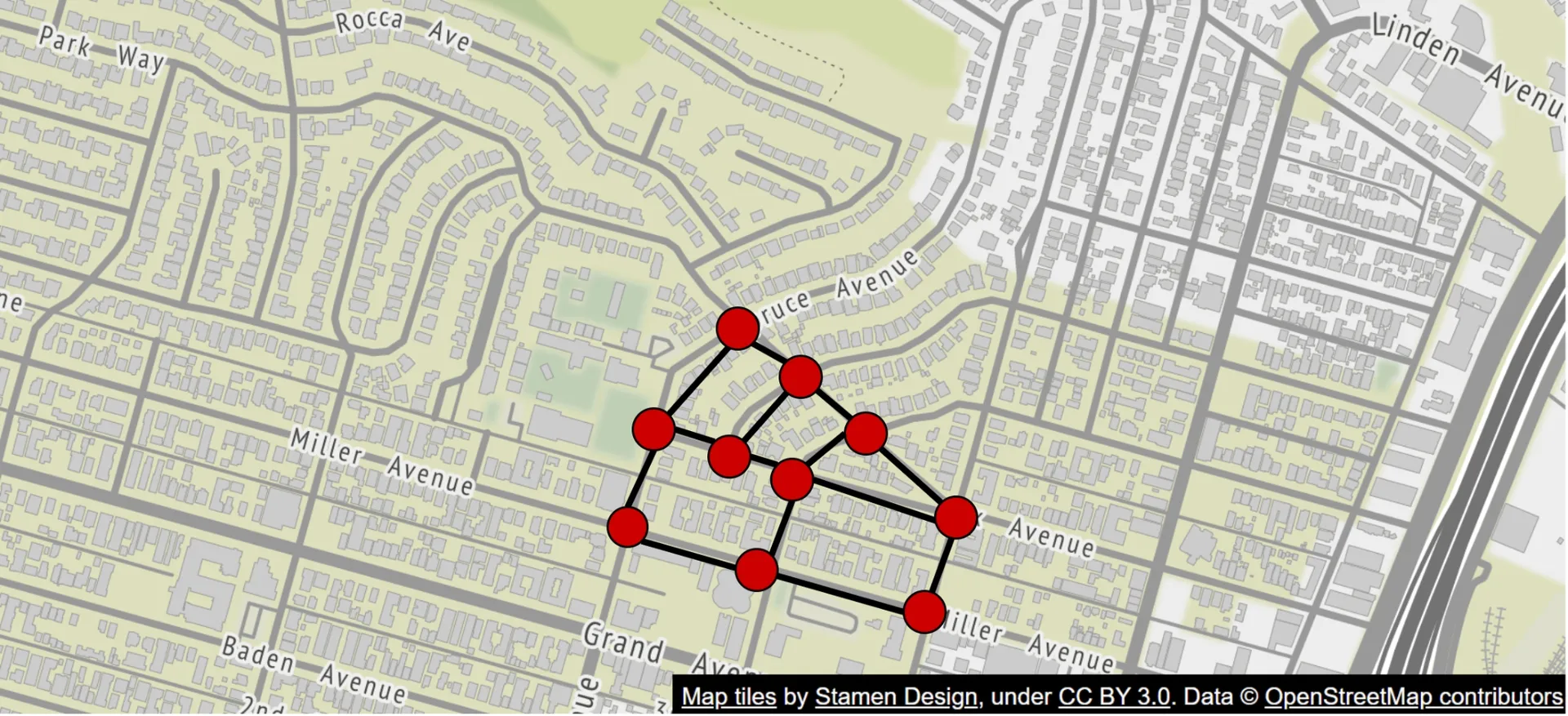
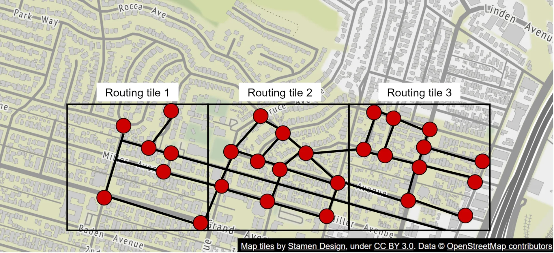
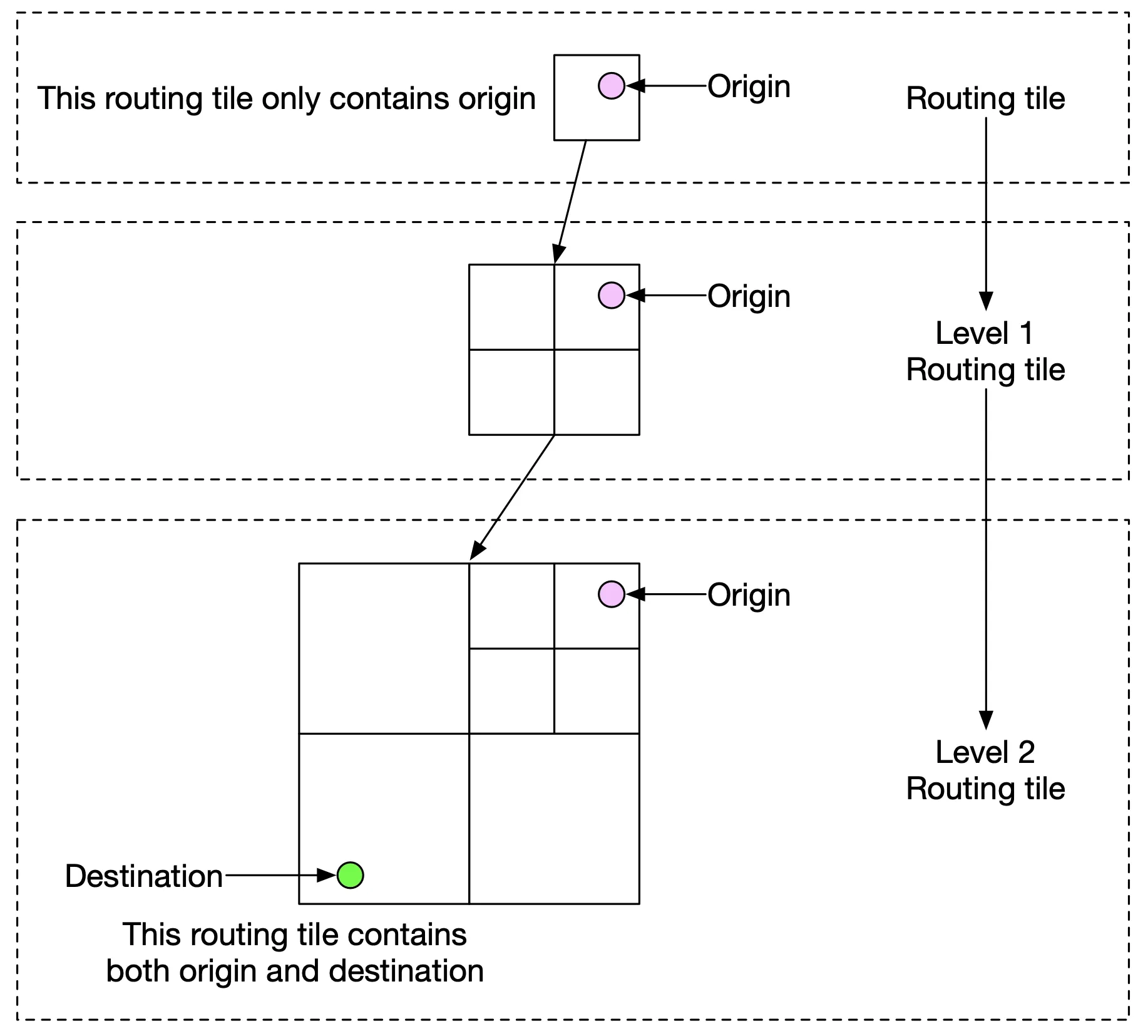
Road data processing for navigation: Routing algorithms (Dijkstra/A* variants) operate on graphs (intersections=nodes, roads=edges). World graph too large → break into routing tiles (binary files of road data per grid). Three hierarchical levels: local roads, arterial roads, major highways. Higher level tiles cover larger areas with fewer details. Tiles reference connected tiles at same/different zoom levels.

Back-of-the-envelope estimation #

Storage (map tiles):

• Zoom level 21: ~4.4 trillion tiles × 100KB = 440 PB raw.
• ~90% is ocean/desert/mountain → highly compressible → reduce 80-90% → ~50 PB at highest zoom.
• Each lower zoom = 4× fewer tiles. Total: 50 + 50/4 + 50/16 + ... = ~67 PB. Rough estimate: ~100 PB for all zoom levels.

Server throughput:

• Navigation: 1B DAU × 5 trips/week ÷ 7 ÷ 10⁵ = ~7,200 QPS (avg). Peak: ~36,000 QPS (5×).
• Location updates: 5B nav minutes/day × 60 = 300B requests/day = 3M QPS (every 1s). Batched every 15s → 200,000 QPS (avg). Peak: ~1M QPS.

Step 2 - Propose High-Level Design and Get Buy-In

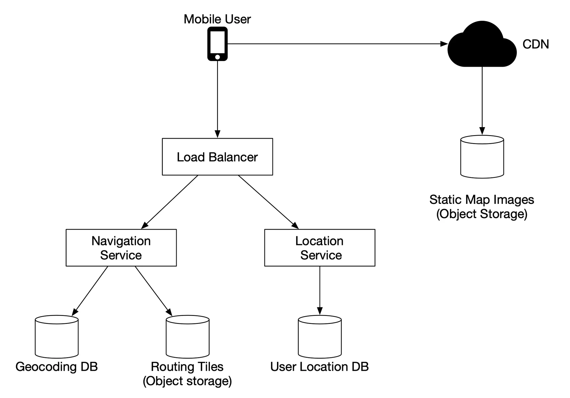
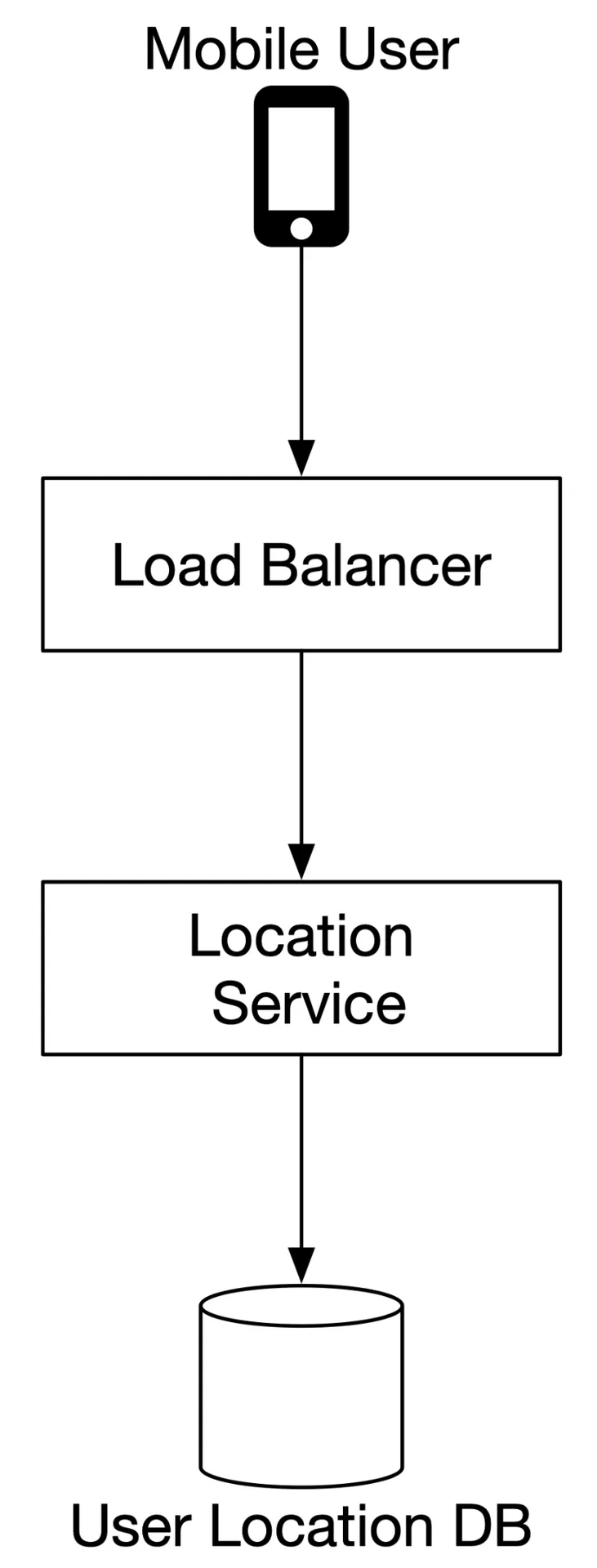
Figure 7 High-level design

Location service #

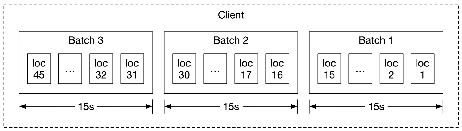
Clients send location updates every X seconds (configurable). Batched: record every 1s, send batch every 15s → reduces traffic. Uses:

• HTTP with keep-alive.
• POST /v1/locations with JSON-encoded array of (lat, lng, timestamp) tuples.
• Database: Cassandra (high write volume, scalable) + Kafka for stream processing.

Navigation service #

Finds a reasonably fast route A→B. Accuracy critical, can tolerate some latency.

• GET /v1/nav?origin=...&destination=...
• Returns: distance, duration, start/end location, polyline, HTML instructions, travel mode.

Map rendering #

Pre-generated static map tiles (option 2) — not dynamically generated. Each tile at a zoom level covers a fixed geohash grid. Served via CDN from nearest POP.

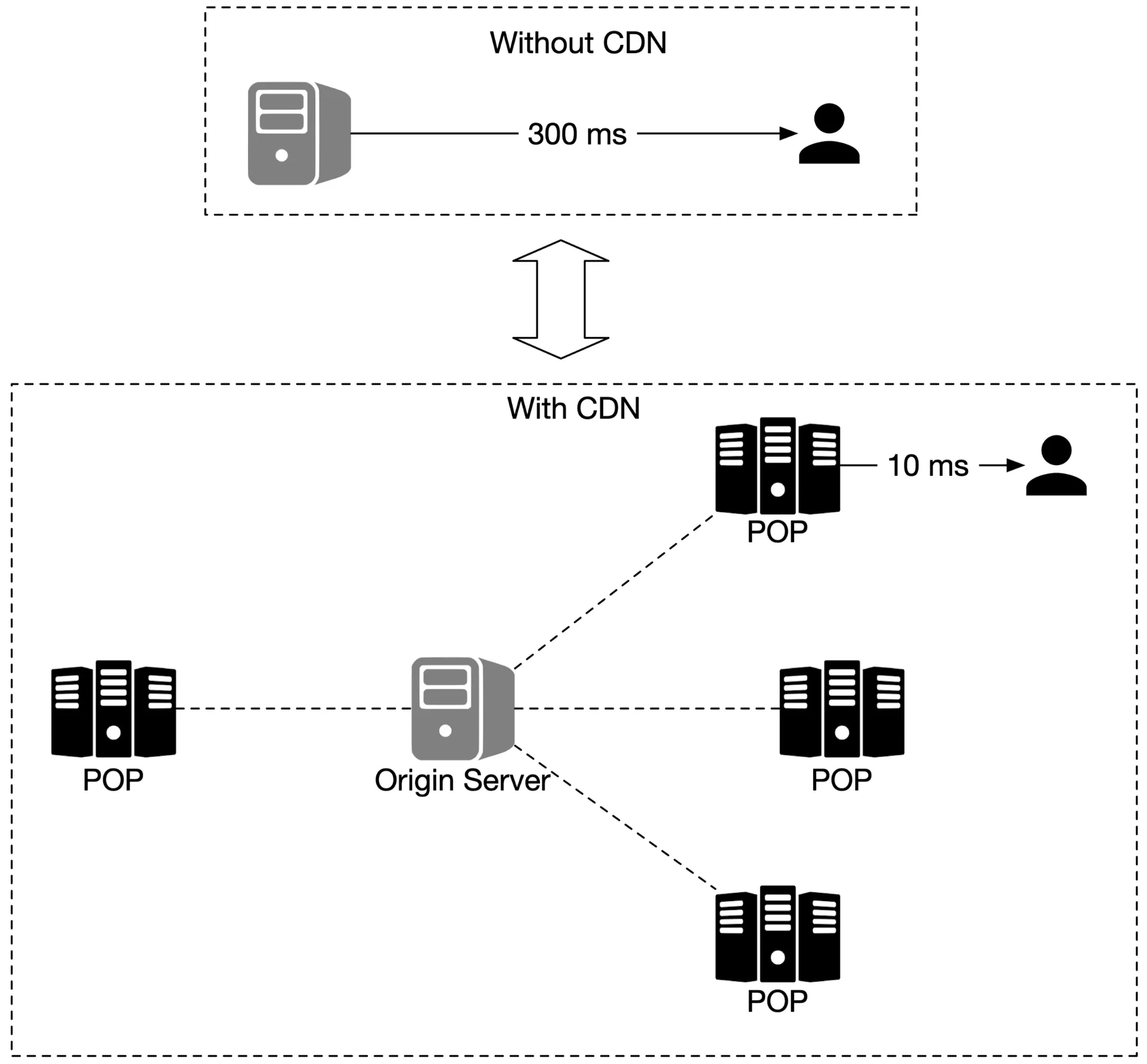
Data usage: At 30km/h, 200m×200m tiles (100KB each), 25 tiles per 1km² = 2.5MB data. → 75MB/hour or 1.25MB/minute.

CDN traffic: 5B nav minutes/day × 1.25MB/min = 6.25B MB/day = ~62,500 MB/sec through CDN. With 200 POPs → few hundred MB/sec each.

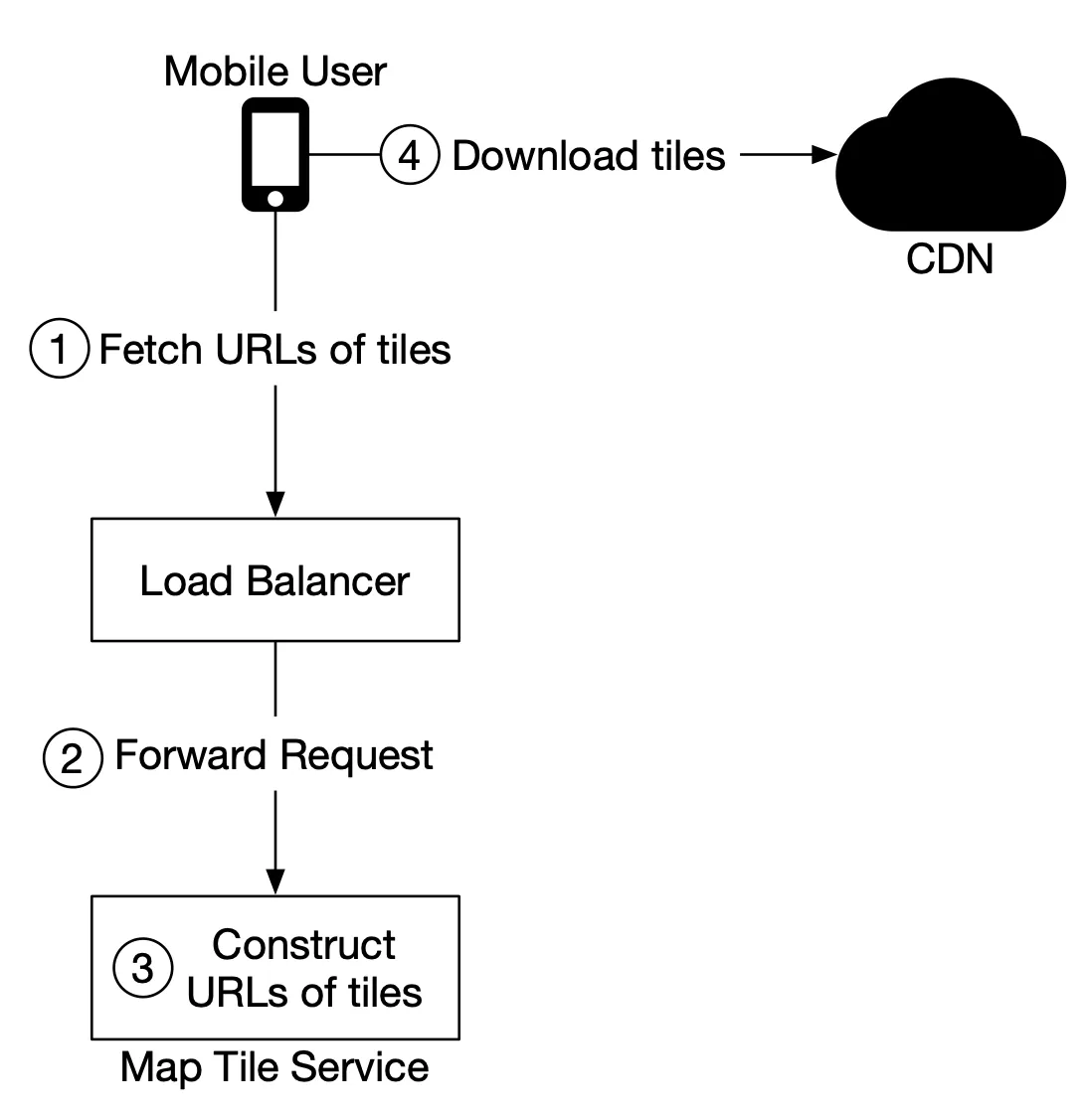
Tile URL construction: Client converts lat/lng + zoom → geohash → URL (e.g., https://cdn.map-provider.com/tiles/9q9heb.png). Alternative: map tile service as intermediary for operational flexibility (avoid hardcoding geohash logic in clients).

Step 3 - Design Deep Dive

Data model #

Routing tiles #

• Raw road data (TBs) → offline routing tile processing service → routing tiles at 3 resolutions.
• Stored as adjacency lists serialized to binary files in object storage (S3), organized by geohash.
• Aggressively cached on routing service. DB not needed.

User location data (Cassandra) #

Partition key: user_id. Clustering key: timestamp. Efficient time-range queries per user. Prioritizes availability over consistency (CAP: AP).

Geocoding database #

Redis key-value store: place → lat/lng. Frequent reads, infrequent writes.

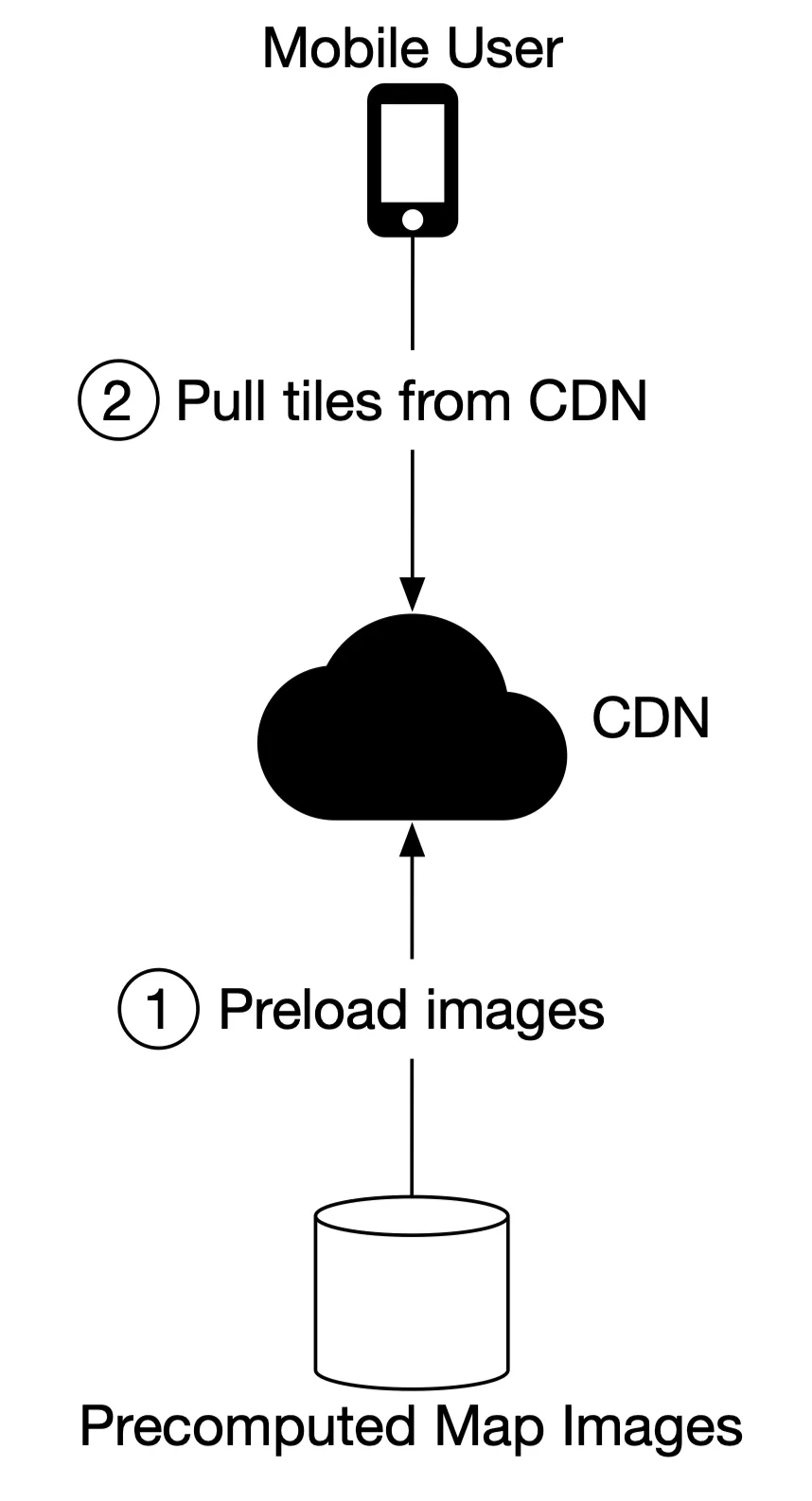
Precomputed map images #

Stored on CDN backed by cloud storage (S3). Precomputed at 21 zoom levels.

Services #

Location service #

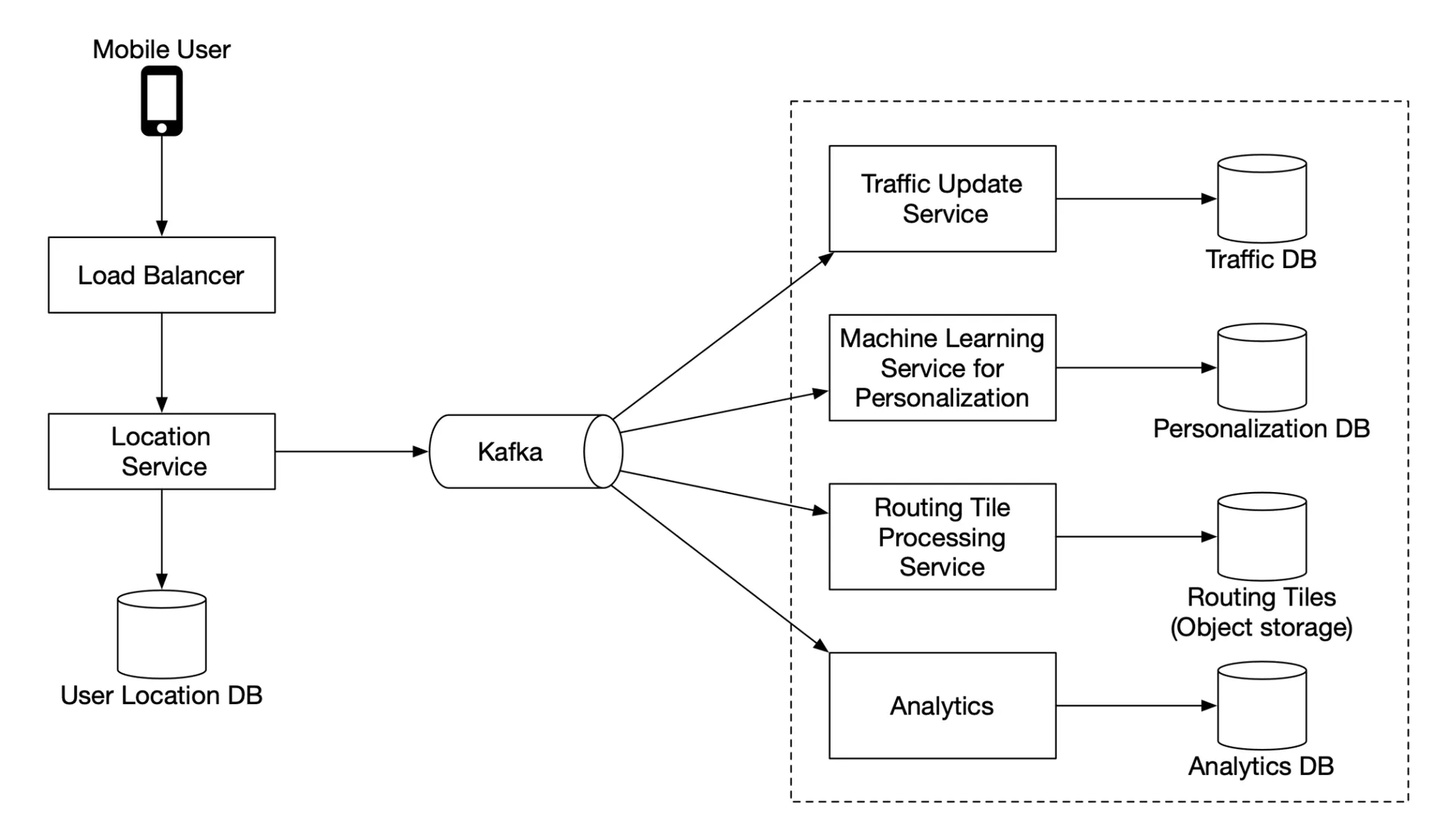
Location data logged to Kafka. Downstream consumers:

• Live traffic service → updates live traffic DB.
• Routing tile processing service → detects new/closed roads, updates routing tiles in object storage.
• Other services tap the stream for various purposes.

Map rendering #

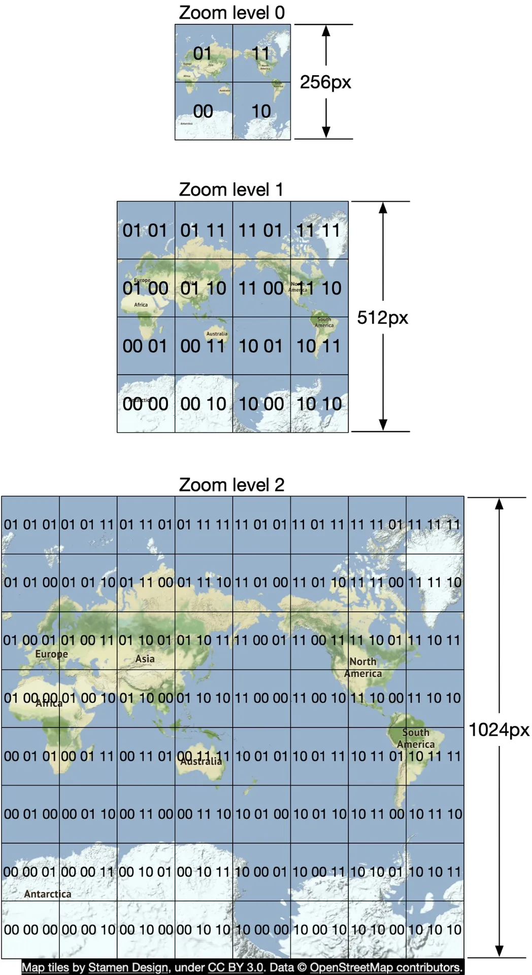
21 zoom levels. Level 0: 1 tile (256×256, entire world). Each increment: 4× tiles, 4× pixels.

Vector optimization: Send vector info (paths, polygons) instead of raster PNGs. Better compression, smoother zooming (no pixelation). Client draws from vectors via WebGL.

Navigation service #

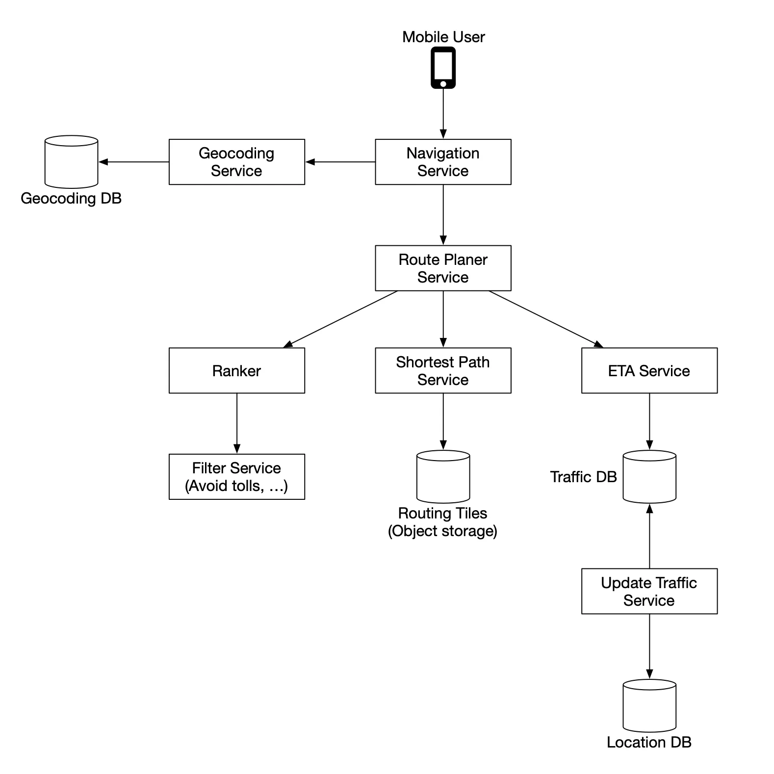
Geocoding service: Resolves address → lat/lng. Uses key-value DB (Redis).

Route planner service: Orchestrates pathfinding.

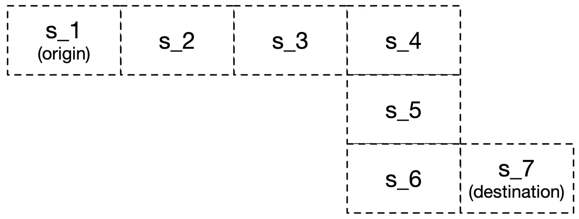
Shortest-path service: A* variant against routing tiles in object storage.

1. Convert origin/destination lat/lng → geohashes → load start/end routing tiles.
2. Traverse graph, load neighboring tiles on demand from object storage (or local cache).
3. Can switch to higher-level tiles (highways) through cross-resolution references.
4. Continue until best routes found.

ETA service: ML-based prediction using current traffic + historical data. Predicts traffic 10-20 min ahead.

Ranker service: Filters routes by user preferences (avoid tolls, avoid freeways), ranks fastest to slowest, returns top-k.

Updater services: Consume Kafka location stream. Traffic update service → live traffic DB. Routing tile processing service → updated routing tiles.

Adaptive ETA and rerouting #

Naive approach: store user → [routing tiles] mapping. Traffic incident on tile s₂ → scan all rows to find affected users. O(n × m) — too slow.

Improved: store user → [current tile, parent tile, grandparent tile]. Check only the largest tile in each row. Fast filtering.

Delivery protocol: WebSocket preferred over mobile push (limited payload, no web support) and long polling. Bi-directional communication supports last-mile delivery. SSE also viable.

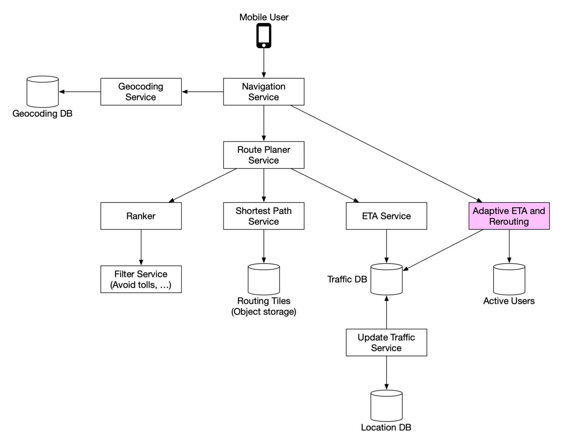
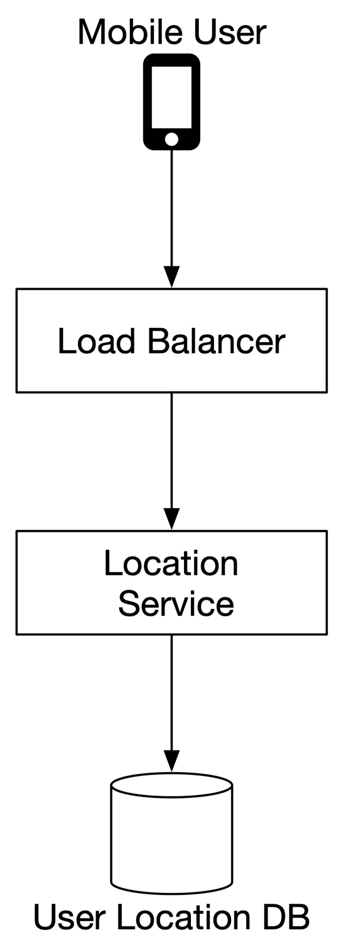
Figure 21 Final design

Step 4 - Wrap Up

Key features: location update (Cassandra + Kafka), ETA/route planning (A* with routing tiles + ML ETA), map rendering (precomputed tiles + CDN + vectors). Adaptive ETA uses hierarchical tile tracking. Multi-stop navigation for enterprise (e.g., delivery services) as potential expansion.